Annotate episodes
annotate_episodes.RmdIntroduction
The chronogram package provides a family of functions to annotate a
chronogram. These all start cg_annotate_. This vignette
explains how to use these annotation functions. Before using this
vignette, consult the vignette("assembly").
Setup
library(chronogram)
library(dplyr)
#>
#> Attaching package: 'dplyr'
#> The following objects are masked from 'package:stats':
#>
#>     filter, lag
#> The following objects are masked from 'package:base':
#>
#>     intersect, setdiff, setequal, union
library(ggplot2)
library(patchwork)
We will use the example pre-built chronogram, introduced in the
vignette("assembly"), and add on some example infection
data.
data(built_smallstudy)
cg <- built_smallstudy$chronogram
infections_to_add <- built_smallstudy$infections_to_add

## add to chronogram
cg <- cg_add_experiment(
  cg,
  infections_to_add
)
Episode annotation
Annotation is required to allow the selection sub-cohorts of individuals (and corresponding dates) that are relevant to test your biological hypothesis.
For episodes, use the cg_annotate_episodes_ family
These perform sequential steps:
-
cg_annotate_episodes_find()is used to identify episodes of infection. This reads across several different experiment data types, that are specified in the function call: eg. symptoms, PCRs, LFTs for SARS-CoV-2. Additionally,cg_annotate_episodes_find()looks backwards and forwards in time to find episodes, as commonly the molecular testing and symptoms do not commence on the same day.
In some studies, seroconversion is the method of finding episodes (eg
seroconversion on anti-N IgG in SARS-CoV-2). Seroconversion episodes can
be found with cg_annotate_episodes_find_seroconversion().
As these provide different (often much, much larger) uncertainty around
the episode start, chronogram handles this in a separate function.
cg_annotate_episodes_fill()allow filling of specific columns for each episode (details below).count the number of episodes (cf
cg_annotate_vaccines_count())
Worked example
The first step is to find episodes using
cg_annotate_episodes_find().
cg_episodes <- cg_annotate_episodes_find(
  cg,
  infection_cols = c("LFT", "PCR", "symptoms"),
  infection_present = c("pos", "Post", "^severe")
)
#> Parsed: infection_cols and infection_present
#>
#> Searching in the [[column]], for the "text":
#> Loading required namespace: stringr
#> stringr::str_detect(.data[["LFT"]], "pos") ~ "yes"
#>
#> stringr::str_detect(.data[["PCR"]], "Post") ~ "yes"
#>
#> stringr::str_detect(.data[["symptoms"]], "^severe") ~ "yes"
#>
#>
#> ...detecting will be exact.
#>           Capitals, spelling etc must be precise
#> Joining with `by = join_by(calendar_date, elig_study_id)`

cg_episodes %>%
  ggplot(
    aes(
      x = calendar_date,
      y = elig_study_id,
      label = episode_number
    )
  ) +
  ## now add text to show when episodes occur ##
  geom_text(
    data = . %>%
      group_by(elig_study_id, episode_number) %>%
      slice_head(),
    col = "red", show.legend = FALSE
  ) +
  theme_bw()
#> Warning: Removed 3 rows containing missing values or values outside the scale range
#> (`geom_text()`).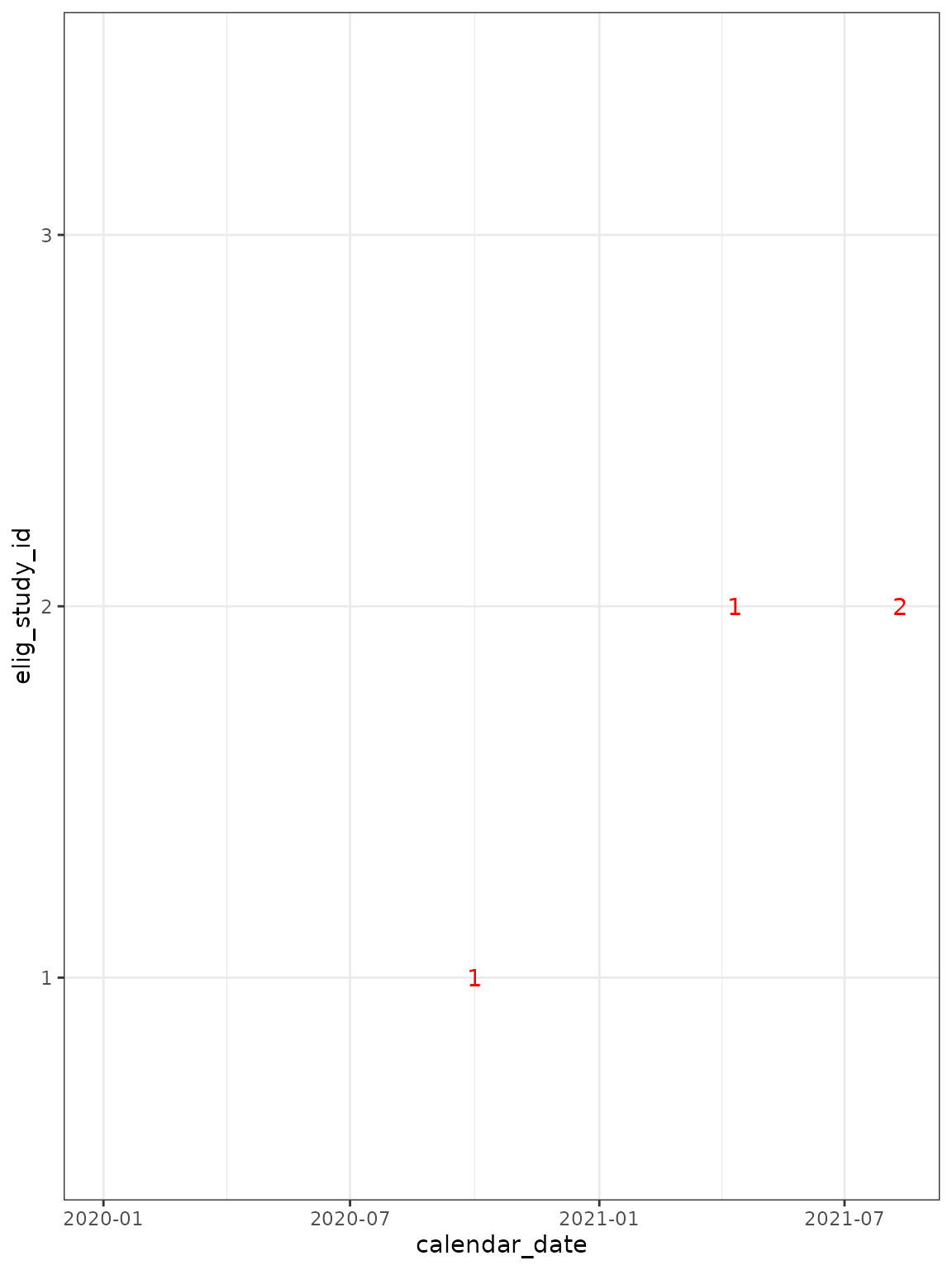
Note that participant 1 has a single infection episode in November 2020, with testing and symptom data on different days:
| calendar_date | elig_study_id | LFT | PCR | symptoms |
|---|---|---|---|---|
| 2020-10-01 | 1 | pos | not tested | NA |
| 2020-10-11 | 1 | pos | NA | severe |
We could use a shorter time frame to look forwards and backwards in:
cg_short_episode_length <- cg_annotate_episodes_find(
  cg,
  infection_cols = c("LFT", "PCR", "symptoms"),
  infection_present = c("pos", "Post", "^severe"),
  ## change episode days interval to 7 days ##
  episode_days = 7
)
#> Parsed: infection_cols and infection_present
#>
#> Searching in the [[column]], for the "text":
#> stringr::str_detect(.data[["LFT"]], "pos") ~ "yes"
#>
#> stringr::str_detect(.data[["PCR"]], "Post") ~ "yes"
#>
#> stringr::str_detect(.data[["symptoms"]], "^severe") ~ "yes"
#>
#>
#> ...detecting will be exact.
#>           Capitals, spelling etc must be precise
#> Joining with `by = join_by(calendar_date, elig_study_id)`

cg_short_episode_length %>%
  ggplot(
    aes(
      x = calendar_date,
      y = elig_study_id,
      label = episode_number
    )
  ) +
  ## now add text to show when episodes occur ##
  geom_text(
    data = . %>%
      group_by(elig_study_id, episode_number) %>%
      slice_head(),
    col = "red", show.legend = FALSE
  ) +
  scale_fill_grey(end = 0.2, start = 0.8) +
  theme_bw()
#> Warning: Removed 3 rows containing missing values or values outside the scale range
#> (`geom_text()`).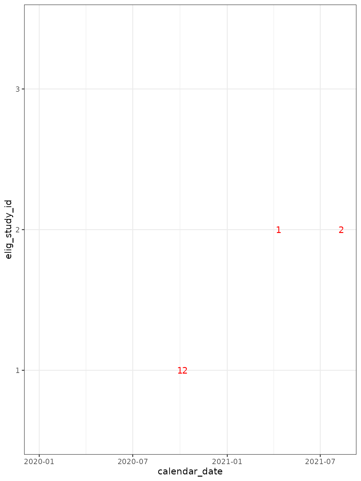
The episode_days option sets the “gap” to look for, rather than the total permitted length of an episode. For example, LFT+ve on d-6, symptoms on d0, and PCR+ on d7 would be collected into a single episode.
Episode variant
Next, we assign variants. There is no one-size-fits all approach that holds across pathogens, across studies, and across geographic regions. In this example we have PCR data available, and could parse as: if there is PCR positivity assign Delta, if there is no PCR testing assign Ancestral/Alpha.
cg_episodes <- cg_episodes %>%
  mutate(
    episode_variant =
      case_when(
        # "is an episode" & "PCR positive" -> Delta #
        (!is.na(episode_number)) & PCR == "Pos" ~ "Delta",
        # "is an episode" & "PCR unavailable" -> Anc/Delta #
        (!is.na(episode_number)) & PCR == "not tested" ~ "Anc/Alpha"
      )
  )
This gives a variant call on a single row of cg.
cg_episodes %>%
  filter(!is.na(episode_variant)) %>%
  pull(episode_variant)
#> [1] "Anc/Alpha" "Anc/Alpha" "Delta"
We can use cg_annotate_episodes_fill() to add this
annotation to every row of the infection episode.
cg_episodes <- cg_episodes %>%
  cg_annotate_episodes_fill(
    col_to_fill = episode_variant,
    col_to_return = episode_variant_filled,
    .direction = "updown",
    episode_numbers_col = episode_number
  )
#> Joining with `by = join_by(elig_study_id, episode_number)`


cg_episodes %>%
  filter(!is.na(episode_variant_filled)) %>%
  pull(episode_variant_filled)
#>  [1] "Anc/Alpha" "Anc/Alpha" "Anc/Alpha" "Anc/Alpha" "Anc/Alpha" "Anc/Alpha"
#>  [7] "Anc/Alpha" "Anc/Alpha" "Anc/Alpha" "Anc/Alpha" "Anc/Alpha" "Anc/Alpha"
#> [13] "Delta"
Variant calling rarely relies on a single assay. We advocate a pragmatic a tiered approach. If viral sequencing results are available we use those; if PCR only (± S gene target failure), we use those; and in the absence of molecular testing we compare episode start dates to prevailing variant trends.
In principle:
each assay result is reported in its own column in 1 (or more) experimental data tibbles
build with
cg_assemble()find episodes as above
fill each of
episode_variant_by_seq,episode_variant_by_PCRandepisode_variant_by_date, and then fill for the whole episode, usingcg_annotate_episodes_fill().write a
case_when()to combine overepisode_variant_by_seq_filled,episode_variant_by_PCR_filledandepisode_variant_by_date_filled. Which result trumps which other results is study-dependent.
… to return a column episode_variant_summarised as the
combined, overall assignment (column naming strategy entirely up to the
user).
Summary
This vignette has provided examples of the cg_annotate family in
action. If you are conducting a multi-pathogen study (RSV, flu, covid),
then run a set of cg_annotate family functions for each pathogen - and
you may wish to prefix the output columns eg RSV_,
flu_ & covid_. As these have differing
considerations for eg variants, chronogram leaves the cg_annotate family
without an overall wrapper to let users easily omit unneeded
annotations.
SessionInfo
sessionInfo()
#> R version 4.4.2 (2024-10-31)
#> Platform: x86_64-pc-linux-gnu
#> Running under: Ubuntu 22.04.5 LTS
#>
#> Matrix products: default
#> BLAS:   /usr/lib/x86_64-linux-gnu/openblas-pthread/libblas.so.3
#> LAPACK: /usr/lib/x86_64-linux-gnu/openblas-pthread/libopenblasp-r0.3.20.so;  LAPACK version 3.10.0
#>
#> locale:
#>  [1] LC_CTYPE=C.UTF-8       LC_NUMERIC=C           LC_TIME=C.UTF-8
#>  [4] LC_COLLATE=C.UTF-8     LC_MONETARY=C.UTF-8    LC_MESSAGES=C.UTF-8
#>  [7] LC_PAPER=C.UTF-8       LC_NAME=C              LC_ADDRESS=C
#> [10] LC_TELEPHONE=C         LC_MEASUREMENT=C.UTF-8 LC_IDENTIFICATION=C
#>
#> time zone: UTC
#> tzcode source: system (glibc)
#>
#> attached base packages:
#> [1] stats     graphics  grDevices utils     datasets  methods   base
#>
#> other attached packages:
#> [1] patchwork_1.3.0  ggplot2_3.5.1    dplyr_1.1.4      chronogram_1.0.0
#>
#> loaded via a namespace (and not attached):
#>  [1] gtable_0.3.6      jsonlite_1.8.9    highr_0.11        compiler_4.4.2
#>  [5] tidyselect_1.2.1  stringr_1.5.1     tidyr_1.3.1       jquerylib_0.1.4
#>  [9] systemfonts_1.1.0 scales_1.3.0      textshaping_0.4.0 yaml_2.3.10
#> [13] fastmap_1.2.0     R6_2.5.1          generics_0.1.3    knitr_1.48
#> [17] tibble_3.2.1      desc_1.4.3        munsell_0.5.1     lubridate_1.9.3
#> [21] bslib_0.8.0       pillar_1.9.0      rlang_1.1.4       utf8_1.2.4
#> [25] stringi_1.8.4     cachem_1.1.0      xfun_0.49         fs_1.6.5
#> [29] sass_0.4.9        timechange_0.3.0  cli_3.6.3         pkgdown_2.1.1
#> [33] withr_3.0.2       magrittr_2.0.3    digest_0.6.37     grid_4.4.2
#> [37] lifecycle_1.0.4   vctrs_0.6.5       evaluate_1.0.1    glue_1.8.0
#> [41] farver_2.1.2      ragg_1.3.3        fansi_1.0.6       colorspace_2.1-1
#> [45] purrr_1.0.2       rmarkdown_2.29    tools_4.4.2       pkgconfig_2.0.3
#> [49] htmltools_0.5.8.1