Quickstart
chronogram.RmdThis vignette is for the impatient and showcases the features of the
chronogram package.
Construct a chronogram
Use cg_assemble() to create a chronogram from cleaned
input data.
## Fictional example data ##
data(smallstudy)


cg <- cg_assemble(
  start_date = "01012020",
  end_date = "10102021",
  ## the provided metadata ##
  metadata = smallstudy$small_study_metadata,
  ## the column name in the metadata that contains participant IDs ##
  metadata_ids_col = elig_study_id,
  ## column name for dates ##
  calendar_date_col = calendar_date,
  ## the provided experiment data (we have 1 assay, so a list of 1) ##
  experiment_data_list = list(smallstudy$small_study_Ab)
)
#> Checking input parameters...
#> -- checking start date 01012020
#> -- checking end date 10102021
#> -- checking end date later than start date
#> -- checking metadata
#> -- checking experiment data list
#> --- checking experiment data list slot 1
#> Input checks completed
#> Chronogram assembling...
#> -- chrongram_skeleton built
#> -- chrongram built with metadata
#> -- adding experiment data
#> --- adding experiment data slot 1 cols... elig_study_id calendar_date serum_Ab_S ...print(), glimpse() and
summary() help explore the resulting chronogram.
(View() works too, but not shown in vignette).
print(cg)
#> # A tibble:     1,947 × 10
#> # A chronogram: try summary()
#>    calendar_date elig_study_id   age sex   dose_1 date_dose_1 dose_2 date_dose_2
#>  * <date>        <fct>         <dbl> <fct> <fct>  <date>      <fct>  <date>
#>  1 2020-01-01    1                40 F     AZD12… 2021-01-05  AZD12… 2021-02-05
#>  2 2020-01-02    1                40 F     AZD12… 2021-01-05  AZD12… 2021-02-05
#>  3 2020-01-03    1                40 F     AZD12… 2021-01-05  AZD12… 2021-02-05
#>  4 2020-01-04    1                40 F     AZD12… 2021-01-05  AZD12… 2021-02-05
#>  5 2020-01-05    1                40 F     AZD12… 2021-01-05  AZD12… 2021-02-05
#>  6 2020-01-06    1                40 F     AZD12… 2021-01-05  AZD12… 2021-02-05
#>  7 2020-01-07    1                40 F     AZD12… 2021-01-05  AZD12… 2021-02-05
#>  8 2020-01-08    1                40 F     AZD12… 2021-01-05  AZD12… 2021-02-05
#>  9 2020-01-09    1                40 F     AZD12… 2021-01-05  AZD12… 2021-02-05
#> 10 2020-01-10    1                40 F     AZD12… 2021-01-05  AZD12… 2021-02-05
#> # ℹ 1,937 more rows
#> # ℹ 2 more variables: serum_Ab_S <dbl>, serum_Ab_N <dbl>
#> # ★ Dates: calendar_date      ★ IDs: elig_study_id
#> # ★ metadata: age, sex, dose_1, date_dose_1, dose_2, date_dose_2

glimpse(cg)
#> Glimpse: chronogram
#>  Dates column:  calendar_date
#>  IDs column:    elig_study_id
#>
#> Metadata
#> Rows: 1,947
#> Columns: 6
#> $ age         <dbl> 40, 40, 40, 40, 40, 40, 40, 40, 40, 40, 40, 40, 40, 40, 40…
#> $ sex         <fct> F, F, F, F, F, F, F, F, F, F, F, F, F, F, F, F, F, F, F, F…
#> $ dose_1      <fct> AZD1222, AZD1222, AZD1222, AZD1222, AZD1222, AZD1222, AZD1…
#> $ date_dose_1 <date> 2021-01-05, 2021-01-05, 2021-01-05, 2021-01-05, 2021-01-0…
#> $ dose_2      <fct> AZD1222, AZD1222, AZD1222, AZD1222, AZD1222, AZD1222, AZD1…
#> $ date_dose_2 <date> 2021-02-05, 2021-02-05, 2021-02-05, 2021-02-05, 2021-02-0…
#>
#> Experiment data & annotations
#> Rows: 1,947
#> Columns: 2
#> $ serum_Ab_S <dbl> NA, NA, NA, NA, NA, NA, NA, NA, NA, NA, NA, NA, NA, NA, NA,…
#> $ serum_Ab_N <dbl> NA, NA, NA, NA, NA, NA, NA, NA, NA, NA, NA, NA, NA, NA, NA,…

summary(cg)
#> A chronogram:
#>  Dates column:  calendar_date
#>  IDs column:    elig_study_id
#>  Starts on:     2020-01-01
#>  Ends on:       2021-10-10
#>  Contains:      3  unique participant IDs
#>  Windowed:      FALSE
#>  Spanning:      649 - 649 days [min-max per participant]
#>  Metadata:      age, sex, dose_1, date_dose_1, dose_2, date_dose_2
#>  Size:          129.55 kB
#>  Pkg_version:   1.0.0 [used to build this cg]
Plot trajectories
Plot antibody responses over time for each individual using
cg_plot().
traj <- cg_plot(cg,
  y_values = serum_Ab_S
)
#> Function provided to illustrate chronogram ->
#>           ggplot2 interface.
#>           Users are likely to want to write their own,
#>           study-specific applications

traj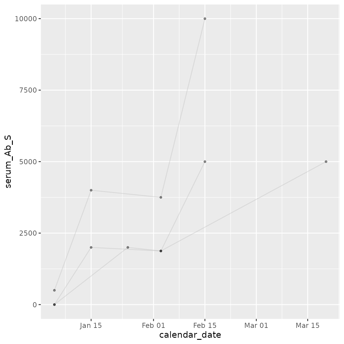
Plot a swimmers plot to visualise an individual’s sequence of events
within the study, using cg_plot_meta().
swimmer <- cg_plot_meta(cg,
  visit = serum_Ab_S
)
#> Function provided to illustrate chronogram ->
#>           ggplot2 interface.
#> Function assumes the
#>           presence of {dose_1, date_dose_1, dose_2, date_dose_2}
#>           columns.
#>           Users are likely to want to write their own,
#>           study-specific applications

swimmer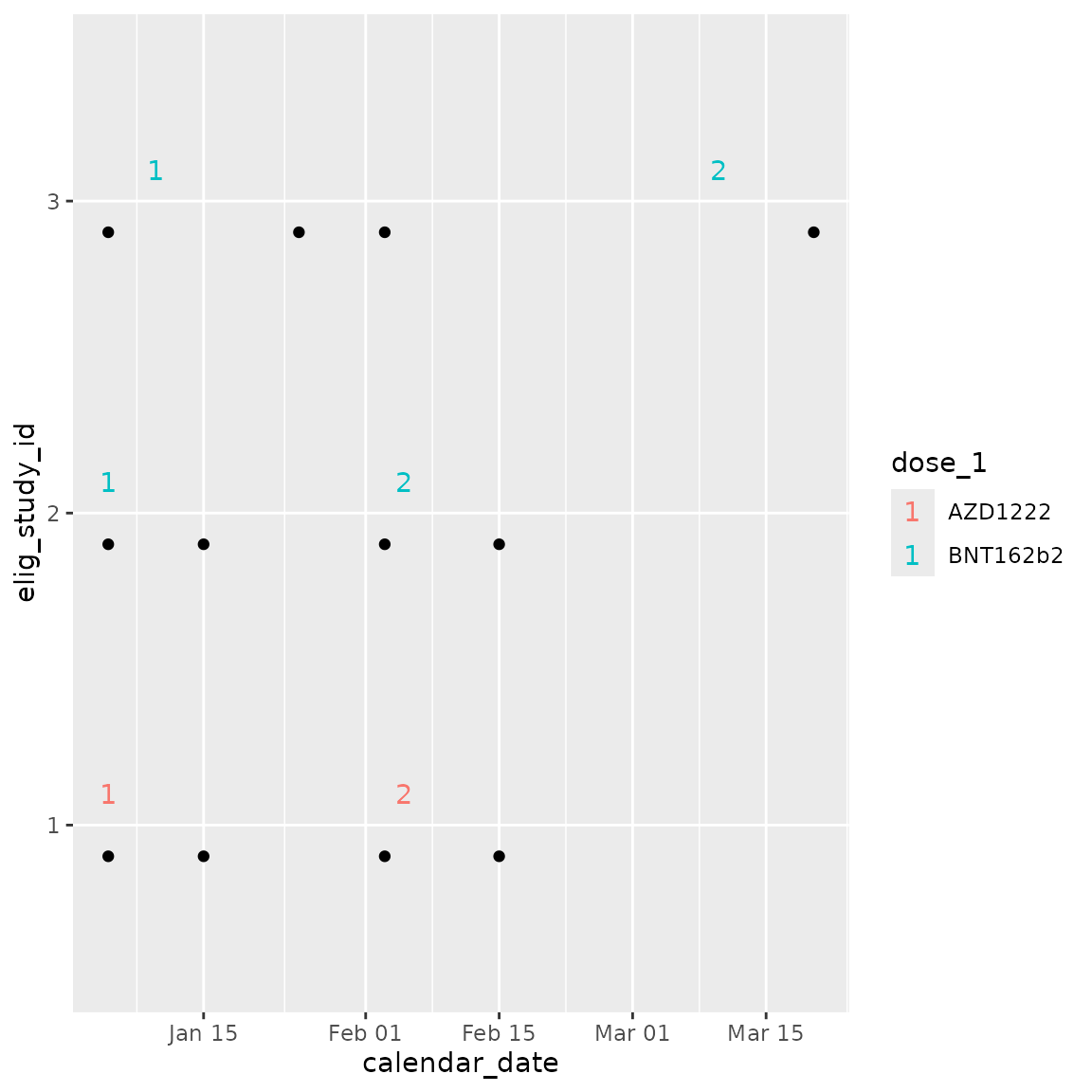
Customise plots
Using ggplot2 or patchwork
customisations.
lay <- "
a
a
a
b
"
(
  (traj + labs(y = "anti-S IgG") + scale_y_log10()) /
    (swimmer + theme(axis.text.y = element_blank()))
) +
  plot_layout(design = lay) &
  plot_annotation(tag_levels = "A") &
  theme_bw(base_size = 8) &
  theme(legend.position = "none") &
  theme(plot.tag = element_text(size = 16, face = "bold")) &
  labs(x = "date")
#> Warning in scale_y_log10(): log-10 transformation introduced infinite values.
#> log-10 transformation introduced infinite values.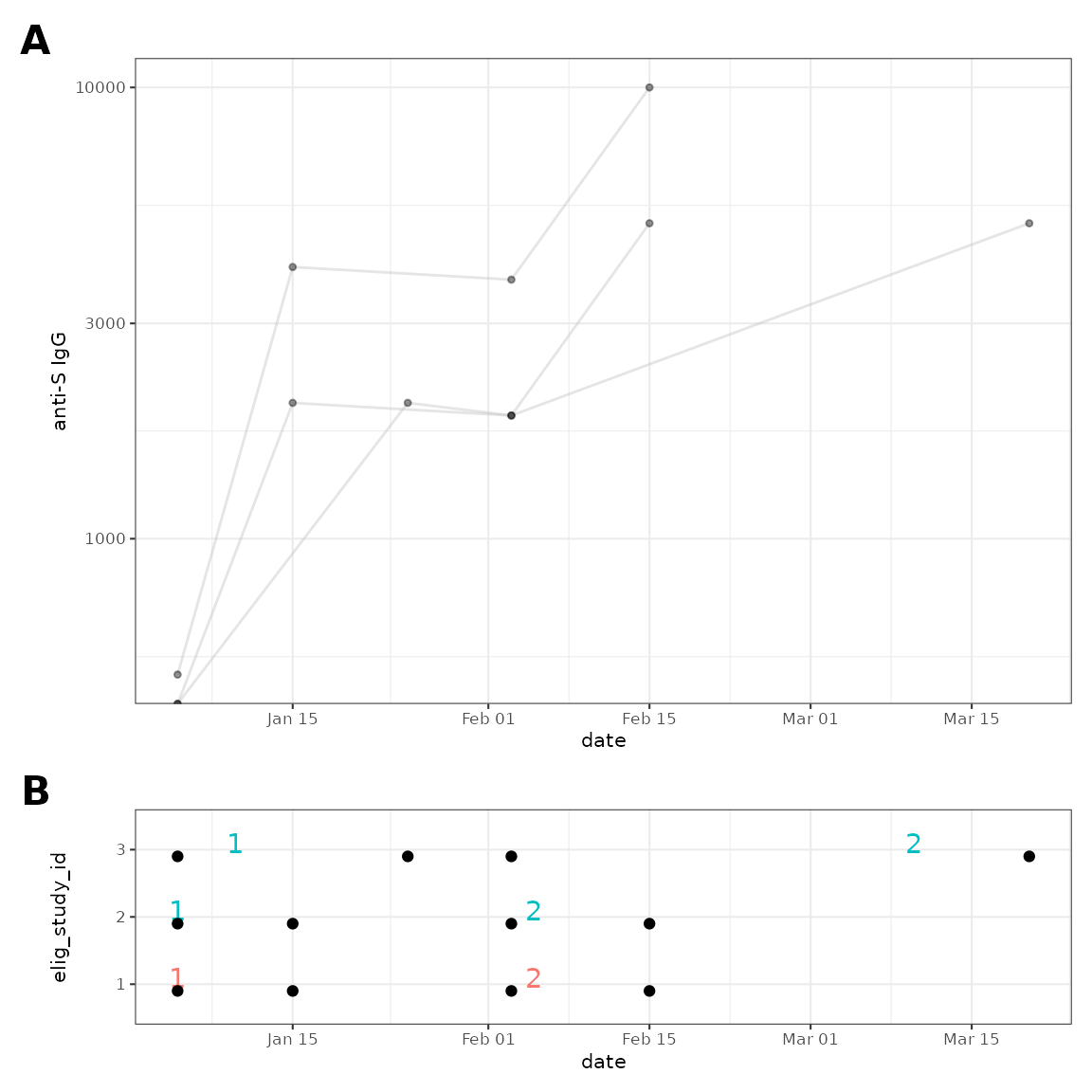
Annotate a chronogram
There are a suite of functions to find, label and count infection episodes. These aggregate across different experiment data columns, such as symptoms, PCRs, viral sequencing. See the annotation vignette.
Window a chronogram
Here, we pick dates in relation to dose 2, using
cg_window_by_metadata().
## upto 50d after dose 2 ##
cg_after_dose_2 <- cg_window_by_metadata(cg,
  windowing_date_col = date_dose_2,
  preceding_days = 0,
  following_days = 50
)

## upto 21d before dose 2 ##
cg_before_dose_2 <- cg_window_by_metadata(cg,
  windowing_date_col = date_dose_2,
  preceding_days = 21,
  following_days = 0
)


cg_after_dose_2 <- cg_after_dose_2 %>% mutate(cohort = "post D2")

cg_before_dose_2 <- cg_before_dose_2 %>% mutate(cohort = "pre D2")

cg_dose_2 <- bind_rows(cg_after_dose_2, cg_before_dose_2)

cg_dose_2 <- cg_dose_2 %>% mutate(
  cohort =
    factor(cohort,
      levels = c(
        "pre D2",
        "post D2"
      )
    )
)
Re-plot the windowed data
traj_2 <- cg_dose_2 %>%
  cg_plot(.,
    y_values = serum_Ab_S
  )
#> Function provided to illustrate chronogram ->
#>           ggplot2 interface.
#>           Users are likely to want to write their own,
#>           study-specific applications

pd <- position_dodge(0.4)

violin_2 <- cg_dose_2 %>%
  ## geom_line fails if lots of NA rows provided ##
  filter(!is.na(serum_Ab_S)) %>%
  ggplot(aes(
    x = cohort, y = serum_Ab_S,
    group = elig_study_id
  )) +
  geom_point(position = pd) +
  geom_line(position = pd)

swimmer_2 <- cg_plot_meta(cg_dose_2,
  visit = serum_Ab_S
)
#> Function provided to illustrate chronogram ->
#>           ggplot2 interface.
#> Function assumes the
#>           presence of {dose_1, date_dose_1, dose_2, date_dose_2}
#>           columns.
#>           Users are likely to want to write their own,
#>           study-specific applications


lay2 <- "
aac
aac
aa#
bb#
"

(
  (traj_2 +
    labs(y = "anti-S IgG", x = "date") +
    scale_y_log10()) +
    (swimmer_2 +
      labs(x = "date") +
      theme(axis.text.y = element_blank())) +
    (violin_2 +
      labs(y = "anti-S IgG") +
      scale_y_continuous(trans = "log10") +
      annotation_logticks(sides = "l"))
) +
  plot_layout(design = lay2) &
  plot_annotation(tag_levels = "A") &
  theme_bw(base_size = 8) &
  theme(legend.position = "none") &
  theme(plot.tag = element_text(size = 16, face = "bold"))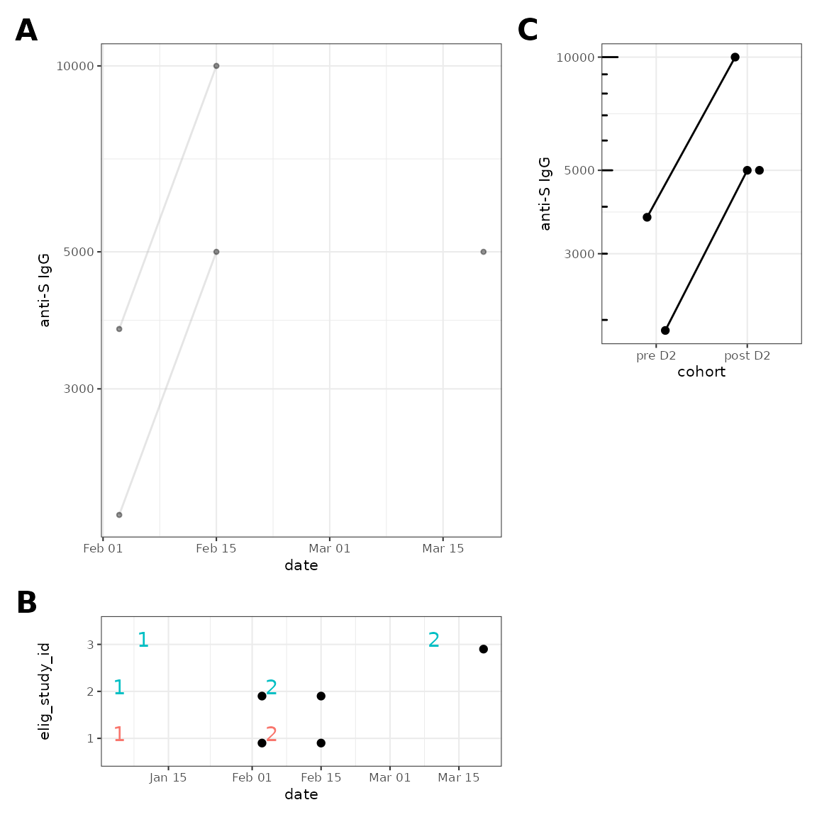
Note that for participant 3, the sample ~50d before dose 2 is now excluded.
Summary
Chronogram is now assembled and the relevant data to answer a (simple) biological question (does dose 2 boost anti-S IgG?) retrieved, plotted and readied for a statistical test.
Please see the other vignettes for a deeper demonstration of chronogram functions.
SessionInfo
sessionInfo()
#> R version 4.4.2 (2024-10-31)
#> Platform: x86_64-pc-linux-gnu
#> Running under: Ubuntu 22.04.5 LTS
#>
#> Matrix products: default
#> BLAS:   /usr/lib/x86_64-linux-gnu/openblas-pthread/libblas.so.3
#> LAPACK: /usr/lib/x86_64-linux-gnu/openblas-pthread/libopenblasp-r0.3.20.so;  LAPACK version 3.10.0
#>
#> locale:
#>  [1] LC_CTYPE=C.UTF-8       LC_NUMERIC=C           LC_TIME=C.UTF-8
#>  [4] LC_COLLATE=C.UTF-8     LC_MONETARY=C.UTF-8    LC_MESSAGES=C.UTF-8
#>  [7] LC_PAPER=C.UTF-8       LC_NAME=C              LC_ADDRESS=C
#> [10] LC_TELEPHONE=C         LC_MEASUREMENT=C.UTF-8 LC_IDENTIFICATION=C
#>
#> time zone: UTC
#> tzcode source: system (glibc)
#>
#> attached base packages:
#> [1] stats     graphics  grDevices utils     datasets  methods   base
#>
#> other attached packages:
#> [1] chronogram_1.0.0 patchwork_1.3.0  ggplot2_3.5.1    dplyr_1.1.4
#>
#> loaded via a namespace (and not attached):
#>  [1] gtable_0.3.6      jsonlite_1.8.9    highr_0.11        compiler_4.4.2
#>  [5] tidyselect_1.2.1  tidyr_1.3.1       jquerylib_0.1.4   systemfonts_1.1.0
#>  [9] scales_1.3.0      textshaping_0.4.0 yaml_2.3.10       fastmap_1.2.0
#> [13] lobstr_1.1.2      R6_2.5.1          labeling_0.4.3    generics_0.1.3
#> [17] knitr_1.48        tibble_3.2.1      desc_1.4.3        munsell_0.5.1
#> [21] lubridate_1.9.3   bslib_0.8.0       pillar_1.9.0      rlang_1.1.4
#> [25] utf8_1.2.4        cachem_1.1.0      xfun_0.49         fs_1.6.5
#> [29] sass_0.4.9        timechange_0.3.0  cli_3.6.3         pkgdown_2.1.1
#> [33] withr_3.0.2       magrittr_2.0.3    digest_0.6.37     grid_4.4.2
#> [37] lifecycle_1.0.4   vctrs_0.6.5       evaluate_1.0.1    glue_1.8.0
#> [41] farver_2.1.2      ragg_1.3.3        fansi_1.0.6       colorspace_2.1-1
#> [45] purrr_1.0.2       rmarkdown_2.29    tools_4.4.2       pkgconfig_2.0.3
#> [49] htmltools_0.5.8.1