Annotate vaccines
annotate_vaccines.RmdIntroduction
The chronogram package provides a family of functions to annotate a
chronogram. These all start cg_annotate_. This vignette
explains how to use these annotation functions. Before using this
vignette, consult the vignette("assembly").
Setup
library(chronogram)
library(dplyr)
#>
#> Attaching package: 'dplyr'
#> The following objects are masked from 'package:stats':
#>
#>     filter, lag
#> The following objects are masked from 'package:base':
#>
#>     intersect, setdiff, setequal, union
library(ggplot2)
library(patchwork)
We will use the example pre-built chronogram, introduced in the
vignette("assembly"), and add on some example infection
data.
data(built_smallstudy)
cg <- built_smallstudy$chronogram
infections_to_add <-  built_smallstudy$infections_to_add

## add to chronogram
cg <- cg_add_experiment(
  cg,
  infections_to_add
)
Vaccine annotation
Annotation is required to allow the selection sub-cohorts of individuals (and corresponding dates) that are relevant to test your biological hypothesis.
For vaccines, use cg_annotate_vaccines_count()
– adds a column which counts the number of vaccines each participant has received over time.
– includes a “star” system, to allow the first few days after a vaccine to be easily identified. For example, 24hrs after the first dose of a vaccine (“1star”) is probably not biologically reflect of that dose’s effect. The user can set the value of days to “star” to suit their analysis.
cg_annotate_vaccines_count() requires that metadata
columns follow this pattern:
dose_1, dose_2, dose_3, …, dose_i
date_dose_1, date_dose_2, date_dose_3, …, date_dose_i
The trailing digit reflects the dose number for both
dose_i and date_dose_i.
The {dose} and {date_dose} prefixes should be provided to the
function, as shown in the chunk below. You might envisage a study with
{sarscov2_dose}, {sarscov2_date_dose}, {influenza_dose} &
{influenza_date_dose} for which two runs of
cg_annotate_vaccines_count() would be needed.
Worked example
cg <- cg_annotate_vaccines_count(
  cg,
  ## the prefix to the dose columns: ##
  dose = dose,
  ## the output column name: ##
  dose_counter = dose_number,
  ## the prefix to the date columns: ##
  vaccine_date_stem = date_dose,
  ## use 14d to 'star' after a dose ##
  intermediate_days = 14
)
#> Using stem: date_dose
#> Found vaccine dates
#> date_dose_1
#>
#> date_dose_2

## plot over time ##
cg %>%
  ggplot(
    aes(
      x = calendar_date,
      y = elig_study_id,
      fill = dose_number
    )
  ) +
  geom_tile(height = 0.5) +
  scale_fill_grey(end = 0.2, start = 0.8) +
  theme_bw()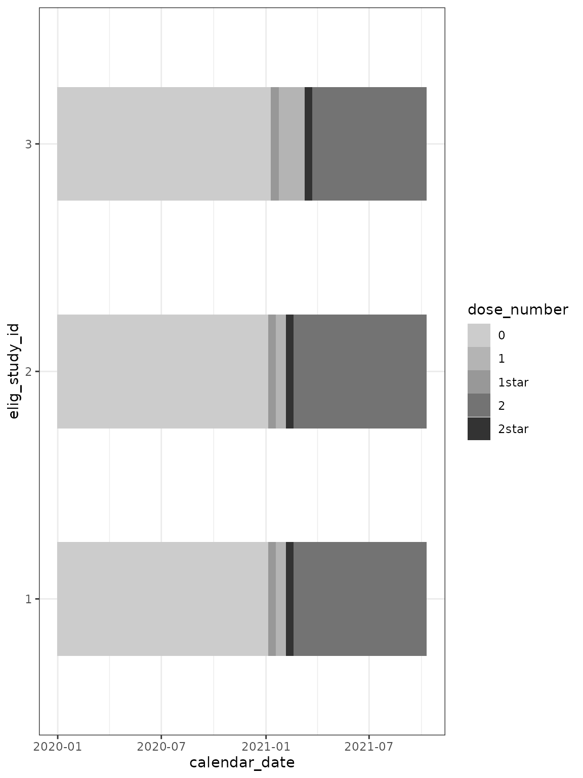
In the above plot, the character vector dose_number is
coerced to a factor. The resulting levels of the factor are
counter-intuitive. To improve the plot, you can manually specify the
factor:
cg %>%
  mutate(dose_number = factor(dose_number,
    levels = c(
      "0",
      "1star",
      "1",
      "2star",
      "2"
    )
  )) %>%
  ggplot(
    aes(
      x = calendar_date,
      y = elig_study_id,
      fill = dose_number
    )
  ) +
  geom_tile(height = 0.5) +
  scale_fill_grey(end = 0.2, start = 0.8) +
  theme_bw()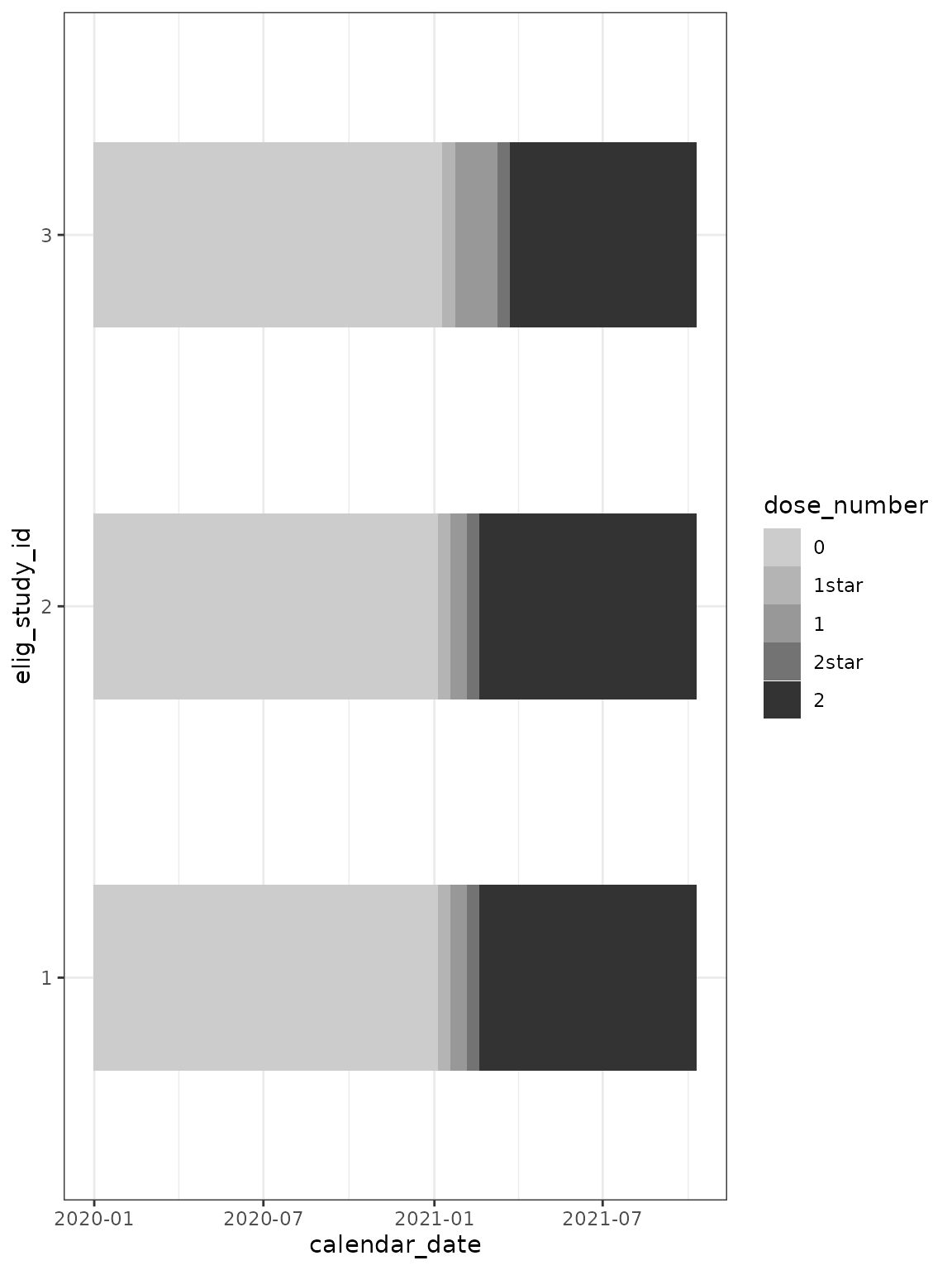
The dose_number column is intentionally returned to
cg as character vector rather than converting to a factor.
There is the possibility for mishandling if a factor:
as.numeric(dose_number) == 1, refers to the situation
dose == 0, and as.numeric(dose_number) == 2,
refers to the situation dose == 1.
Summary
This vignette has provided examples of the cg_annotate family in
action. If you are conducting a multi-pathogen study (RSV, flu, covid),
then run a set of cg_annotate family functions for each
pathogen - and you may wish to prefix the output columns eg
RSV_, flu_ & covid_.
SessionInfo
sessionInfo()
#> R version 4.4.2 (2024-10-31)
#> Platform: x86_64-pc-linux-gnu
#> Running under: Ubuntu 22.04.5 LTS
#>
#> Matrix products: default
#> BLAS:   /usr/lib/x86_64-linux-gnu/openblas-pthread/libblas.so.3
#> LAPACK: /usr/lib/x86_64-linux-gnu/openblas-pthread/libopenblasp-r0.3.20.so;  LAPACK version 3.10.0
#>
#> locale:
#>  [1] LC_CTYPE=C.UTF-8       LC_NUMERIC=C           LC_TIME=C.UTF-8
#>  [4] LC_COLLATE=C.UTF-8     LC_MONETARY=C.UTF-8    LC_MESSAGES=C.UTF-8
#>  [7] LC_PAPER=C.UTF-8       LC_NAME=C              LC_ADDRESS=C
#> [10] LC_TELEPHONE=C         LC_MEASUREMENT=C.UTF-8 LC_IDENTIFICATION=C
#>
#> time zone: UTC
#> tzcode source: system (glibc)
#>
#> attached base packages:
#> [1] stats     graphics  grDevices utils     datasets  methods   base
#>
#> other attached packages:
#> [1] patchwork_1.3.0  ggplot2_3.5.1    dplyr_1.1.4      chronogram_1.0.0
#>
#> loaded via a namespace (and not attached):
#>  [1] gtable_0.3.6      jsonlite_1.8.9    highr_0.11        compiler_4.4.2
#>  [5] tidyselect_1.2.1  stringr_1.5.1     tidyr_1.3.1       jquerylib_0.1.4
#>  [9] systemfonts_1.1.0 scales_1.3.0      textshaping_0.4.0 yaml_2.3.10
#> [13] fastmap_1.2.0     R6_2.5.1          generics_0.1.3    knitr_1.48
#> [17] tibble_3.2.1      desc_1.4.3        munsell_0.5.1     lubridate_1.9.3
#> [21] bslib_0.8.0       pillar_1.9.0      rlang_1.1.4       utf8_1.2.4
#> [25] stringi_1.8.4     cachem_1.1.0      xfun_0.49         fs_1.6.5
#> [29] sass_0.4.9        timechange_0.3.0  cli_3.6.3         pkgdown_2.1.1
#> [33] withr_3.0.2       magrittr_2.0.3    digest_0.6.37     grid_4.4.2
#> [37] lifecycle_1.0.4   vctrs_0.6.5       evaluate_1.0.1    glue_1.8.0
#> [41] farver_2.1.2      ragg_1.3.3        fansi_1.0.6       colorspace_2.1-1
#> [45] purrr_1.0.2       rmarkdown_2.29    tools_4.4.2       pkgconfig_2.0.3
#> [49] htmltools_0.5.8.1