cg_plot_meta

Create a ggplot2 object, plotting a user-defined metadata over time in a swimmer's plot.

ggplot2 objects retain the entirety of the provided dataset. This allows later adjustments, such as adding extra geom_layers with new information, or applying facets. To find this data examine obj$data. If you save ggplot2 objects, all source data is ALSO saved. cg_plot_meta() removes any un-used data by default (drop_vars=TRUE). In writing a study specific ggplot2, it is best practice to select minimal columns before calling ggplot().

Usage

cg_plot_meta(
  cg,
  x = NULL,
  date_dose_1 = date_dose_1,
  dose_1 = dose_1,
  date_dose_2 = date_dose_2,
  dose_2 = dose_2,
  visit = visit,
  drop_vars = TRUE,
  fill = NULL
)

Arguments

cg

chronogram

x

a column of time to use as x axis. If NULL, will default to the chronogram's calendar date attribute. A user may want to derive and use alternatives eg 'daysSinceDose2'.

date_dose_1

column containing the date of dose.

dose_1

column containing the vaccine formulation.

date_dose_2

column containing the date of dose.

dose_2

column containing the vaccine formulation.

visit

column within chronogram to indicate a study visit (i.e. samples available; NA when samples not taken, !=NA when samples available). In our small study example, serum_Ab_S fills this brief.

drop_vars

Default TRUE. See description.

fill

column used to determine fill

Examples

library(ggplot2)
library(patchwork)

data("built_smallstudy")
cg <- built_smallstudy$chronogram

p1 <- cg_plot_meta(cg,
  visit = serum_Ab_S
)
#> Function provided to illustrate chronogram ->
#>           ggplot2 interface.
#> Function assumes the
#>           presence of {dose_1, date_dose_1, dose_2, date_dose_2}
#>           columns.
#>           Users are likely to want to write their own,
#>           study-specific applications

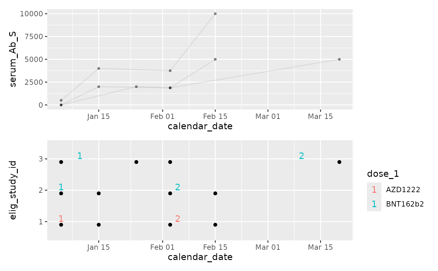
p2 <- cg_plot(cg,
  y_values = serum_Ab_S
)
#> Function provided to illustrate chronogram ->
#>           ggplot2 interface.
#>           Users are likely to want to write their own,
#>           study-specific applications

p2 / p1


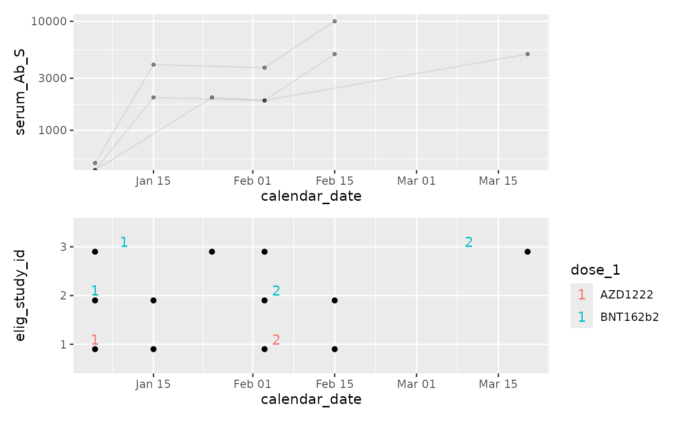
(p2 + scale_y_log10()) / p1
#> Warning: log-10 transformation introduced infinite values.
#> Warning: log-10 transformation introduced infinite values.